What is Verilog?

Verilog is a Hardware Description Language (HDL). It is not a sequential programming language like C.

For example, consider this C code which would be executed line-by-line:

    int j=0;
    int k=1;
    int l=0;
    for (int i=0; i<6; i=i+1) {
        l = k;
        k = j + k;
        j = l;
    }

The variables are updated one at a time in each clock cycle:

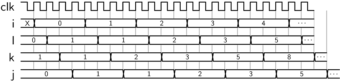
Modules and Circuits

An HDL describes hardware entities or modules that have their own separate existence, and interact via signals. The flow of signals is handled by registers which are updated synchronously by a master clock signal.

Data Flow Example

Suppose each of the modules implements an integer addition function: q := a + b, and all registers are initialized with a value of one.

Describing the Circuit in Verilog

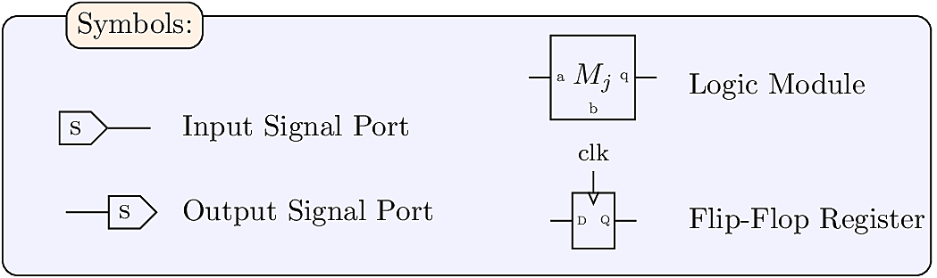
Verilog supports modeling at several levels of abstraction, which include:

Physical circuits (with electrical characteristics and delays)
Structural circuits (describe schematic connections)
Behavioral models (describe functional characteristics)
Test and verification (many functions and tools similar to C libraries)

Modern digital designs are modeled at the Register Transfer Level (RTL), which primarily employs behavioral models that are synthesizable, and may also include structural hierarchies.

Synthesizable RTL Design

RTL designs use a synthesizable subset of behavioral syntax.

Synthesizable syntax examples:

   b <= a;              // Simple assignment
   
   a <= a + b;          // Basic arithmetic
   
   if (a > 0)  b <= a;  // Conditional logic
   else        b <= 1;

Non-synthesizable syntax examples:

   real a, b;    // Real numbers work in simulation, not synthesis
   
   #10 b = a;         // Delay 10 ``time units'' before assignment
   
   $display("%f", b); // Like printf, displays values in the console

Non-synthesizable syntax is useful for testbenches, but doesn’t translate to hardware.

RTL Example

Here’s a synthesizable behavioral model of our example module:

module M(clk, b);
    input            clk;
    output reg [7:0] b;
    
    reg [7:0] a;
    
    initial begin
        a = 1;
        b = 1;
    end
    
    always @(posedge clk) begin
        a <= a + b;
        b <= a;
    end
endmodule

Let’s go through this line by line.

Module declarations

module M(clk, b);
   input            clk;
   output reg [7:0] b;

Begins with the module keyword.
The parentheses contain a comma-separated list of I/O signal ports.
Terminated with a semicolon.
Port direction, type, and bit-width are defined on the following lines.

Alternative Port Declaration

An alternative syntax declares the I/O port types:

module M(
   input            clk, 
   output reg [7:0] b
   );

Port direction, type, and bit-width are defined within the module declaration.
This style is considered more readable, but less compact.

I/O Ports: direction and type

Every I/O port needs a defined direction, either input or output (or inout in special cases).
I/O ports are signals. Every signal needs a type.
The default type is a single-bit wire.

This line declares clk as one input wire:

input            clk;

I/O Ports: Bus Declaration

The next line declares an 8-bit bit vector or bus:

output reg [7:0] b;

The reg keyword declares that signal ‘b’ will be defined as part of a hardware behavioral model, to be assigned within always or initial scopes (more on that later).
The brackets [7:0] declare a bus with wires indexed from 7 down to 0, giving a total of eight.

Internal Signals

In addition to I/O ports, most modules also need internal signals.

reg [7:0] a;

Signal a is not accessible outside the module, so is declared “internally.”
Again the keyword reg indicates that a is used in a hardware behavioral model.
The signal is an 8-bit bus.

Behavioral Models: Initialization

Verilog allows an initial statement to define the initial values of reg signals.

initial
    begin
        a = 1;
        b = 1;
    end

In Xilinx FPGAs, the initial statement is synthesizable – it defines the powerup states of actual hardware signals.
Multiple lines are grouped between begin and end statements.
Initial assignments are made with the ‘=’ operator, and every line is terminated with a semicolon.
WARNING: initial statements are not officially synthesizable. This code will work with Xilinx FPGAs, but to make portable RTL code that can be used with other tools and devices, you should define an explicit reset input and associated reset behavior to replicate the initial conditions.

Version with Reset

The code below modifies our example to include a reset input.

module M(clk, rst_n, b);
    input            clk;
    input            rst_n;
    output reg [7:0] b;
    
    reg [7:0] a;
    
    always @(posedge clk, negedge rst_n) begin
       if (~rst_n) begin
          a <= 1;
          b <= 1;
        end
        else begin
           a <= a + b;
           b <= a;
        end
    end
endmodule

Reset Considerations

Reset signals are conventionally active low. Since a device will typically power-up with low-level signals (until something pulls them high), this helps ensure that it starts in the reset state.
In our example, the always block is sensitive to negedge rst_n, meaning it is evaluated when rst_n falls to zero, and the assignments are executed when rst_n is low:

always @(posedge clk, negedge rst_n) begin
       if (~rst_n) begin
          ...
        end

The subscript _n is used here to indicate that the signal is active-low. This is done to make the code easier to understand.
This code demonstrates an asynchronous reset, since the reset code is evaluated the instant rst_n changes, regardless of what’s happening with the clock signal. This can be important for powerup reset, since the system can reset before the clock ever starts.

Behavioral Models: Synchronous Logic

Behavioral models are defined using the always keyword.

always @(posedge clk) begin
        a <= a + b;
        b <= a;
    end

The always keyword must be followed by a sensitivity list beginning with an ‘@’ sign.
For synchronous (i.e. clocked) logic, sensitivity is either posedge or negedge. In this case, the behavior is actuated on the rising edge (posedge) of clk.
To make synchronous assignments, the <= operator is used. This assignment has a special meaning:
- The assignment will be completed after the clock edge.
- On the right side of the operator, the operations are computed before the clock edge.

Behavioral Models: Combinational Logic

As an alternative syntax style, we can use a combinational model to make the circuit more explicit:

    
    // COMBINATIONAL LOGIC:
    reg [7:0] q;
    
    always @(a,b) begin
        q = a + b;  // Blocking assignment 
    end
    
    // SEQUENTIAL LOGIC:
    always @(posedge clk) begin
        a <= q;    // Non-blocking assignments 
        b <= a;
    end

In combinational models, the sensitivity list must reference all dependencies for the assignments, in this case a and b.
Alternatively a wildcard can be used: always @(*)
Combinational assignments like q = a+b are blocking, interpreted line-by-line.
Clocked assignments like b <= a are non-blocking, interpreted concurrently with other lines in the group.

Behavioral Models: Continuous Assignments

As yet another alternative syntax style, we can declare q as a wire (as opposed to reg) and use the assign statement to define its combinational behavior:

    
    // COMBINATIONAL LOGIC:
    wire [7:0] q;
    
    assign q = a + b;  // continuous assignment 
    
    // SEQUENTIAL LOGIC:
    always @(posedge clk) begin
        a <= q;    // Non-blocking assignments 
        b <= a;
    end

This syntax provides a compact way to represent simple combinational assignments.

Blocking vs Non-Blocking: Unstable Feedback

Consider this modified version that uses only blocking combinational assignments:

    reg [7:0] q;
    
    // COMBINATIONAL LOGIC:
    always @(*)
       q = a + b;  
       a = q;    
       b = a;
    end

Within the always @(*) scope, each line is interpreted as a physical connection, like this:

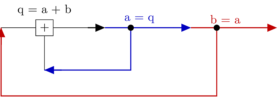
This circuit has direct wired feedback, but nothing to regulate timing. The only stable solution is q == a == b == 0.

Blocking vs Non-Blocking: Stable Timed Feedback

Our original design uses a mix of blocking and non-blocking assignments.

    always @(a,b) begin
        q = a + b;  // Blocking assignment 
    end

    always @(posedge clk) begin
        a <= q;    // Non-blocking assignments 
        b <= a;    // create registers
    end

Each non-blocking assignment, when sensitive to posedge clk, implies a clocked D register, so data is processed on a controlled schedule.

End of the Module

A module concludes with the endmodule statement. It should appear by itself on a line with no semicolon:

endmodule

After the endmodule statement, you can define additional modules in the same file if desired.

Expression Syntax: Bitwise Operators

These operators are applied pairwise across all bits in a vector.

& AND
| OR
^ XOR
~ NOT

Expression Syntax: Bitwise Operators

Example using continuous assignment:

  input [7:0] a;
  input [7:0] b;

  wire [7:0] q;

  assign q = a & b;

The output is:

  q[0] = a[0] & b[0] 
  q[1] = a[1] & b[1]
  q[2] = a[2] & b[2]
  ... and so on.

Expression Syntax: Bitwise Operators

Example with reg signal:

  input [7:0] a;
  input [7:0] b;

  reg [7:0] q;

  always @(*) begin
     q = a & b;
  end

This is essentially the same as the assign example.

Expression Syntax: Replication and Concatenation

{a,b} concatenate a and b into one vector
{N{b}} repeat N copies of b

example:

    input [7:0] a;
    input       b;
    wire  [7:0] q;
    
    assign q = a & {7{b}};

The output is

  q[0] = a[0] & b 
  q[1] = a[1] & b
  q[2] = a[2] & b
    ...  and so on.

Expression Syntax: Logical vs Binary

A logical expression is defined as a Verilog statement that is “true” or “false”.
This is not precisely the same as binary signal values 0 or 1.

Examples:

Expression	Type	Value
`a`	binary signal	`1`
`b`	binary signal	`0`
`a & b`	bitwise operation	`0`
`a == 1`	logical expression	true
`b == 1`	logical expression	false

Expression Syntax: Logical Operators

Logical operators are used for conditional expressions. In the syntax below, the term “exp” refers to any logical expression.

a == b true if a equals b
a != b true if a doesn’t equal b
exp2 && exp2 true if exp1 AND exp2 are true
exp2 || exp2 true if exp1 OR exp2 are true
!exp true if exp is false

Bitwise operators can be used in conditional expressions, but is bad style. Logical operators can be used in assignments, but is usually bad style.

Expression Syntax: Conditionals

if-else statements are supported for reg signals within always or initial scope blocks.
Can be used within combinational or sequential logic.

  input      [2:0] a;
  output reg       b;
  
  always @(a) begin
     if (a>2)
        b = 0;
     else 
        b = 1;
  end

Expression Syntax: Conditionals

expr ? true_assignment : false_assignment is supported for wire signals in continuous assignments.

  input      [2:0] a;
  output           b;
  
  assign b = (a>2) ? 0 : 1;

Expression Syntax: Conditionals

case statements are supported for reg types in always scope blocks:

  input      [2:0] a;
  output           b;
  
  always @(a) begin
    case (a)
      0:       b = 0;
      1:       b = 0;
      2:       b = 0;
      default: b = 1;
    endcase
  end

Inferred Latches Important!!

In combinational logic models:

Every if should have an else
Every case should have a default assignment.

Otherwise you will imply that the signal is stored in a latch, which is usually not what you want. Consider this example:

  input      [2:0] a;
  output reg       b;
  
  always @(a) begin
     if (a>2)
        b = 0;
     else if (a==2)
        b = 1;
  end

What happens when a is less than 2?

Four-Valued Logic: Signals

Verilog signals are binary, but can take four values:

0 Driven to logic low
1 Driven to logic high
X Unknown or invalid signal
Z Not driven (high impedance, floating, or disconnected)

Four-Valued Logic: Bitwise Operators

When the inputs contain X or Z values, bitwise operations use an extended definition as shown in the truth tables below. Notice that when Z is an input, the output can still be a valid logic level, or can be X.

Four-Valued Logic: Comparison Operators

Is this expression true or false?

      (4'b10X1 == 4'b1011)

In Verilog, this comparison returns X, neither true nor false, because one of the digits is unknown.
To include X and Z values in the comparison, use the triple-equal operator (===).

     (4'b10X1 === 4'b1011) (returns false)
     (4'b10X1 === 4'b10X1) (returns true)

Similarly, to check inequality:

     (4'b10X1 !== 4'b1011) (returns true)
     (4'b10X1 !== 4'b10X1) (returns false)

Arithmetic Operations

a + b Integer Addition
a - b Integer Subtraction
a * b Integer Multiplication (complex circuit)
a / b Integer Division (not synthesizable!)
a % b Integer Modulo (not synthesizable!)
a << b Shift bits left
a >> b Shift bits right

Testing and Verification

Testbenches

Most of the time, code should be tested in simulation before implementing it in hardware. A testbench is a module that does the following:

Instantiate the design under test (DUT).
Generate clock and reset signals.
Create stimulus signals for all the DUT inputs.
Perform verification tasks to ensure the DUT does what is expected.

A testbench module typically has no input or output ports. Automated verification may be done by comparing the DUT signals against a “golden” model of the intended design. Manual verification may be done by delivering information to the user via the console or output files.

Example Testbench Module

Here is an example testbench for our design:

module testbench();
    reg          clk;
    reg          rst;
    wire  [7:0]  b;
    integer      clock_count;
    
    M DUT (
       .clk(clk),
       .rst(rst),
       .b(b)
     );
     
    initial begin
       clk         = 0;
       rst         = 0;  // Startup in reset
       clock_count = 0;
       
       forever #10 clk = ~clk; // Create clock signal
    end
    
    always @(posedge clk) begin
       clock_count <= clock_count + 1;
       if (clock_count > 0)
          rst <= 1;  // End reset after one clock cycle
    end
endmodule

Useful Testbench System Tasks

There are several non-synthesizable $ commands called system tasks that are useful for verification and debugging:

$display Like printf, used to print information to the console.
$stop Like a breakpoint, pauses simulation.
$finish Ends simulation completely.
$reset Restart simulation from time zero.
$random Generate a random integer.

Example for our testbench:

always @(posedge clk) begin
       clock_count <= clock_count + 1;
       if (clock_count == 1)
          rst <= 1;  // End reset after one clock cycle
       else if (clock_count == 18)
     $finish;
       
       $display("%d\t%d\t%d",clock_count,rst,b);     
    end

Like in the C printf function, ‘\t’ indicates a tab, and %d indicates a decimal value.

Note on Simulating Examples

When simulating small example designs, it is often more convenient to run terminal simulations rather than create a full Vivado project. Suppose your design files are in a directory named “example_design”, and the files are named “M.v” and “testbench.v”. Open a terminal, change to that directory, and run these commands:

    [example_design/]$ xvlog M.v testbench.v
    [example_design/]$ xelab --debug typical testbench -s sim
    [example_design/]$ xsim --runall sim

The first command, xvlog, compiles your code and reports any syntax errors. If your design uses all the Verilog files in the directory, you can specify *.v instead of listing the files. The second command, xelab, analyzes the hierarchy and reports any connection problems or undefined modules. You specify the top-level module name (“testbench” in this example), and provide a simulation name (“sim”). The final command, xsim, runs the simulation. The –runall argument tells it to run in batch mode; make sure your testbench has a $finish command so that it knows when to stop.

Simulating with Cadence Incisiv

When you are on campus, you can utilize a faster and more powerful simulation tool from Cadence Design Systems. This tool is widely used in industry for designing electronic chips and systems. Our university license only allows it to be used on-site. To use the Cadence simulator, you need to add the tool’s directory to the PATH environment variable. To do this, launch a text editor like gedit and open the file named .bashrc in your home directory. Add this line to the end of the file:

   export PATH=/opt/cadence/installs/INCISIV152/tools/bin:$PATH

Save the file, then launch a new terminal. Now you can use the irun command to compile, elaborate and simulate all in one step:

    [example_design/]$ irun M.v testbench.v

This usually runs much faster than the Xilinx tools, and gives you a chance to test your code on different platforms.

Testbench `$display` Output

Running this testbench with our module yields the output shown at right. The columns are:

clock_count
rst
b

As expected, the rst signal starts at 0 and rises to 1 in the next cycle after clock_count equals 1. Then b starts accumulating after another cycle delay (remember that <= assignments have a clock delay, because they load data into flip-flops that activate on the clock edge).

Notice that we have an overflow condition at clock_count 16. This is because we only allocated 8 bits to our signals, so the highest they can count is 255. We will revisit this problem shortly.

  clock_count  rst    b
  -----------  ---   ----
          0     0      1
          1     0      1
          2     1      1
          3     1      1
          4     1      2
          5     1      3
          6     1      5
          7     1      8
          8     1     13
          9     1     21
         10     1     34
         11     1     55
         12     1     89
         13     1    144
         14     1    233
         15     1    121
         16     1     98 <== ovf
         17     1    219

Alternative: `$strobe` Output

Instead of using $display, we can use a similar command called $strobe. It has the same syntax, but whereas $display shows values just before the clock edge, $strobe shows values just after the clock edge, i.e. after all the synchronous assignments are completed.

The difference is subtle. In this example it just means we start on clock_count 1 instead of 0.

 clock_count  rst    b
 -----------  ---   ----
          1    0      1
          2    1      1
          3    1      1
          4    1      2
          5    1      3
          6    1      5
          7    1      8
          8    1     13
          9    1     21
         10    1     34
         11    1     55
         12    1     89
         13    1    144
         14    1    233
         15    1    121
         16    1     98
         17    1    219
         18    1     61

Alternative `$write` Output

Another task with the same syntax is $write. The only difference is that $display adds a newline, and $write doesn’t. This can be useful for printing arrays, or for splitting complicated displays onto several lines, like in the example code below.

   always @(posedge clk) begin
       clock_count <= clock_count + 1;
       if (clock_count == 1)
          rst <= 1;  
       else if (clock_count == 18)
       $finish;
       
       $write("%d\t",clock_count);
       $write("%d\t",rst);
       $write("%d\n",b);
    end

 clock_count  rst    b
 -----------  ---   ----
          0    0      1
          1    0      1
          2    1      1
          3    1      1
          4    1      2
          5    1      3
          6    1      5
          7    1      8
          8    1     13
          9    1     21
         10    1     34
         11    1     55
         12    1     89
         13    1    144
         14    1    233
         15    1    121
         16    1     98
         17    1    219

File Input and Output

Suppose instead of writing to the console, we want to write to a file. To do this, we can open a file using the $fopen task, and print text data using the $fwrite task. The $fwrite task has essentially the same syntax as $write:

integer f;  // File identification number

initial begin
    f = $fopen("output.txt","w"); // open "output.txt" for writing
    clk         = 0;
    rst         = 0;  // Startup in reset
    clock_count = 0;
       
    forever #10 clk = ~clk; // Create clock signal
end

always @(posedge clk) begin
    // Write a line to the file:
    fwrite(f,"%d\t$d\t%d\n",clock_count,rst,b);

    // Keep track of time, decide when to quit:
    clock_count <= clock_count + 1;
    if (clock_count == 1)
        rst <= 1;  // End reset after one clock cycle
    else if (clock_count == 18) begin
        $fclose(f); // Close file when done
        $finish;
    end

end

Reusability, Portability, Readability

Parameters Within a module definition, you can declare parameters to make the module more flexible. The code below works exactly the same as our original version, but now the width can be adjusted. With a width of 8 bits, the maximum value is 255. We might need to support larger numbers in some applications. Using a parameter makes it easy to adjust.

module M(clk, b);
   parameter WIDTH=8;
   
    input                  clk;
    output reg [WIDTH-1:0] b;
    
    reg        [WIDTH-1:0] a;
    
    initial begin
        a = 1;
        b = 1;
    end
    
    always @(posedge clk) begin
        a <= a + b;
        b <= a;
    end
endmodule

``define, localparam, param`

There are several different ways to define parameters:

`define: global constants and macros

// WIDTH will be the same everywhere in the design
`define WIDTH 8

module M(clk, b);
    output reg [WIDTH-1:0] b;
    //...
endmodule

Note that this command uses a “back tick” located at the upper left of the keyboard.

``define, localparam, param`

parameter: constants can be modified for each module instance:

module M(clk, b);

    // WIDTH will be constant only within each instance
    parameter WIDTH = 8;

    output reg [WIDTH-1:0] b;
    //...
endmodule

``define, localparam, param`

We can instantiate two M modules with different WIDTHs:

module testbench();
    //...
    
    // Instance "DUT1" has WIDTH 8
    M #(.WIDTH(8)) DUT1  (
      .clk(clk),
      .rst(rst),
      .b(b1)
     );

    // Instance "DUT2" has WIDTH 16
    M #(.WIDTH(16)) DUT2  (
      .clk(clk),
      .rst(rst),
      .b(b2)
     );
     
     //...
endmodule

Parameter values can be modified in the instance declaration using the syntax:

 <module_type> #(<parameter_list>) <instance_name> (<port_list>);

``define, localparam, param`

If we add the 16-bit signal, b2, to the output data file, we see that the overflow does not occur at clock-count 16:

clock_count    rst    b1 (8bit)   b2 (16bit)
===========    ===    =========   ==========
          0     0         1         1
          1     0         1         1
          2     1         1         1
          3     1         1         1
          4     1         2         2
          5     1         3         3
          6     1         5         5
          7     1         8         8
          8     1        13        13
          9     1        21        21
         10     1        34        34
         11     1        55        55
         12     1        89        89
         13     1       144       144
         14     1       233       233
         15     1       121       377
         16     1        98       610   <==== b1 overflows, not b2
         17     1       219       987

``define, localparam, param`

localparam: constant within module, not changeable

module M(clk, b);

    // WIDTH will be constant in all instances of M
    localparam WIDTH = 8;
    
    output reg [WIDTH-1:0] b;
    //...
endmodule

Tasks

A task is sort of like a module within a module. Tasks are used to package lines of code that will be reused multiple times. For example, suppose we need to reverse the bit-order of some signals:

module my_interface (
  output reg  [7:0] out1,
  output reg  [7:0] out2,
  input       [7:0] sig1,
  input       [7:0] sig2
);
  integer i;

   always @(sig1,sig2) begin
     reverse_bits(sig1,out1);  // Makes code more compact,
     reverse_bits(sig2,out2);  // improves readability
   end

   task reverse_bits(
      input [7:0] sig,
    output  [7:0]  out
   );
           
    begin
      for (i=0; i<8; i=i+1)
         out[7-i] = sig[i];
    end
   endtask // reverse_bits
   
endmodule

Task Example Testbench

module testbench();
    reg          clk;
    reg   [7:0]  sig1;
    reg   [7:0]  sig2;
    wire  [7:0]  out1;
    wire  [7:0]  out2;
   
    my_interface DUT1 (
       .sig1(sig1),
       .sig2(sig2),
       .out1(out1),
       .out2(out2)
     );
     
    initial begin
       clk   = 0;
       sig1  = 0;
       sig2  = 8'hFF;
       
       // Print column headers on the terminal:
       $write("  sig1  \t  sig2  \t  out1  \t  out2\n");
       $write("  ====  \t  ====  \t  ====  \t  ====\n");

       forever #10 clk = ~clk; // Create clock signal
    end
    
    //...continued on next slide...

Task Example Testbench (continued)

always @(posedge clk) begin
       sig1 <= sig1 + 1;  // sig1 counts up from zero
       sig2 <= sig2 - 1;  // sig2 counts down to zero
       
       if (sig2 == 0)
          $finish;
       
       // Print signal values on the terminal:
       $write("%b\t",sig1);
       $write("%b\t",sig2);
       $write("%b\t",out1);
       $write("%b\n",out2);       
    end
endmodule

Task Example Output

  sig1        sig2        out1        out2
  ====        ====        ====        ====
00000000    11111111    00000000    11111111
00000001    11111110    10000000    01111111
00000010    11111101    01000000    10111111
00000011    11111100    11000000    00111111
00000100    11111011    00100000    11011111
00000101    11111010    10100000    01011111
00000110    11111001    01100000    10011111
00000111    11111000    11100000    00011111

Functions

Functions are like tasks, with a couple of differences:

Functions return a single value.
Function calls look like this:
out_signal = function_name(in1, in2, ...);
Tasks allow timing syntax (#delays, posedge, negedge).
Functions do not.
Functions can call other functions, but cannot call tasks.
Functions can model combinational logic assignments.

Functions vs Tasks

The main differences are:

	task	function
Multi output	Y	N
Timing Statements	Y	N
Consumes time	Y	N
inout ports	Y	N
output ports	Y	N
can call tasks	Y	N
can call functions	Y	Y
returns a value	N	Y

Tasks are versatile, but functions can be safer since they do not affect timing.

Function Example

Here is our task example, rewritten as a function:

module my_interface (
  output reg  [7:0] out1,
  output reg  [7:0] out2,
  input       [7:0] sig1,
  input       [7:0] sig2
);

   always @(sig1,sig2) begin
      out1 = reverse_bits(sig1);
      out2 = reverse_bits(sig2);      
   end

   function [7:0] reverse_bits;
      input [7:0] sig;
      integer i;
      begin
        for (i=0; i<8; i=i+1)
           reverse_bits[7-i] = sig[i];
        end
    endfunction // reverse_bits
   
endmodule

ECE 3700: Verilog Syntax Review Intro to RTL Design

What is Verilog?

Modules and Circuits

Data Flow Example

Describing the Circuit in Verilog

RTL Basics

Synthesizable RTL Design

Non-synthesizable syntax examples:

RTL Example

Module declarations

Alternative Port Declaration

I/O Ports: direction and type

I/O Ports: Bus Declaration

Internal Signals

Behavioral Models: Initialization

Version with Reset

Reset Considerations

Behavioral Models: Synchronous Logic

Behavioral Models: Combinational Logic

Behavioral Models: Continuous Assignments

Blocking vs Non-Blocking: Unstable Feedback

Blocking vs Non-Blocking: Stable Timed Feedback

End of the Module

Verilog Expressions

Expression Syntax: Bitwise Operators

Expression Syntax: Bitwise Operators

Expression Syntax: Bitwise Operators

Expression Syntax: Replication and Concatenation

Expression Syntax: Logical vs Binary

Expression Syntax: Logical Operators

Expression Syntax: Conditionals

Expression Syntax: Conditionals

Expression Syntax: Conditionals

Inferred Latches Important!!

Four-Value Logic

Four-Valued Logic: Signals

Four-Valued Logic: Bitwise Operators

Four-Valued Logic: Comparison Operators

Arithmetic

Arithmetic Operations

Testing and Verification

Testbenches

Example Testbench Module

Useful Testbench System Tasks

Note on Simulating Examples

Simulating with Cadence Incisiv

Testbench $display Output

Alternative: $strobe Output

Alternative $write Output

File Input and Output

Reusability, Portability, Readability

`define, localparam, param

`define, localparam, param

`define, localparam, param

`define, localparam, param

`define, localparam, param

Tasks

Task Example Testbench

Task Example Testbench (continued)

Task Example Output

Functions

Functions vs Tasks

Function Example

ECE 3700: Verilog Syntax Review

Intro to RTL Design

Testbench `$display` Output

Alternative: `$strobe` Output

Alternative `$write` Output

``define, localparam, param`

``define, localparam, param`

``define, localparam, param`

``define, localparam, param`

``define, localparam, param`